How Hypothetical Recreated Welikia
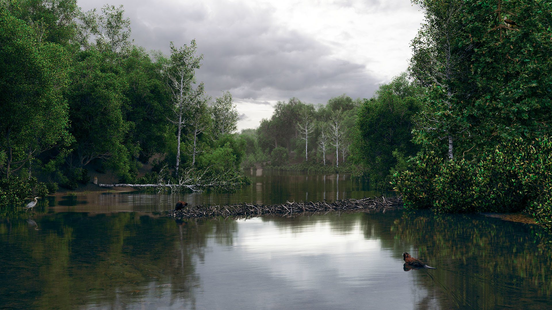
Hypothetical recently wrapped up the first phase of our digital recreation of Welikia and I’m excited to share some information about how it was done. This project is a collaboration with the Wildlife Conservation Society. Dr. Eric Sanderson and his team at the WCS spent years developing extensive ecological models of New York City before European settlement – when it was a diverse and rich array of ecosystems.


Production Requirements
There were a number of requirements for the project in addition to the core need to create photorealistic images based on their data. In fact the images were meant to be the output of a system for interpreting the underlying data, not just a one-off set of scenes and images. For that system we wanted to accomplish a number of goals:
- make it easy enough for a non-expert user to create images
- allow viewpoints from anywhere, roughly categorized as nadir (satellite) views, aerial views and ground level views
- allow for a user, or a scripted solution, to input latitude and longitude coordinates for the camera location
- for the nadir views, be able to render the terrain in tiles to allow for the images to be used in multi-resolution map browsers like Open Street Map
- represent a wide variety of ecosystems and their specific vegetation species
- not be limited to only still images but also allow for animation and panoramic images
- accommodate future updates to the data as more research is completed
These requirements, combined with the scope of the terrain – the data covered 230 square miles (596 square kilometers) of visible landscape and another 470 square miles (1217 square kilometers) of data underwater – and a need for detailed control over how the landscapes are generated meant a standard off-the-shelf solution wouldn’t be suitable.
Based on my experience working with Gaffer I thought it would be an excellent solution. Combined with some data preprocessing in Houdini, our Gaffer script was able to check all the boxes.
Data Preparation
The data I got from Dr. Sanderson’s team was in the form of raster and vector GIS (Geographic Information System) data. Raster data is an image where each pixel, or cell, encodes information for that grid point. Elevation data encodes height above sea level. Ecosystems are identified by a numeric code for the most likely ecosystem for that area based on Dr. Sanderson’s ecological modeling. Vector data described things like pond outlines and Lenape trails.
Some early experiments showed that the resolution of the elevation data held up great at long and medium view distances, but ground level views didn’t have as much detail as we wanted. To improve that I run the elevation data through Houdini’s terrain tools to add a mild erosion effect at an upsampled resolution of 1m per pixel instead of 5m per pixel. This is also where I bring in the vector data through a custom Houdini node for reading the supplied shapefile vector data to ensure ponds contained water. The same scheme is used to cut streams into the terrain by “dredging” a little bit of terrain and prepping Houdini to treat it as water.
Now I have a set of images with elevation and water depth encoded in the pixels. That, the ecosystem raster data and a variety of tree and plant models made with SpeedTree will bring Welikia to life.
Building the World
To keep all of the requirements above met, I decided to structure the overall model as a single world that can be viewed through cameras free to move anywhere in space. It is procedurally created and populated with vegetation, but there is only ever one definitive distribution of plants. This makes it possible to render seamless tiles that line up correctly for nadir views and explore the world with cameras without limitation.
Gaffer’s easy customization and open access to its source code makes creating new nodes in either c++ or Python accessible and greatly extends the ability to tailor just the right solution.
Terrain
At 1m resolution and approximately 58,000m x 55,000m dimensions (once the supplied raster data was squared off) the whole terrain doesn’t have a chance of fitting into memory for rendering. So I break it up into a set of 1024 tiles instead of one huge raster file.
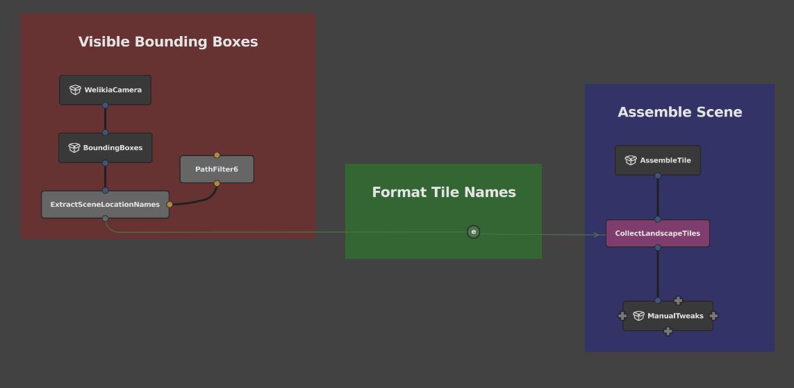
Gaffer has a really great method for assembling scenes with its CollectScenes node. I give that node a list of tiles to include and the upstream tile assembly nodes result in a nice orderly scene graph. The list of tiles to assemble comes from a couple of nodes I created. One takes a scene consisting of bounding boxes for the whole set of terrain tiles and prunes the boxes that are outside of the camera frustum from the scene graph. A second node extracts the names of the scene locations that are still present and turns them into a simple string list that is sent to the CollectScenes node via an expression.
Upstream from the CollectScenes node is a plane with grid divisions of at least 1m spacing. I created a new Gaffer node for sampling image data onto a 3d mesh in order to transfer the height values from the raster images to the 3d grid points and an OSLObject node to displace the points vertically according to the elevation.
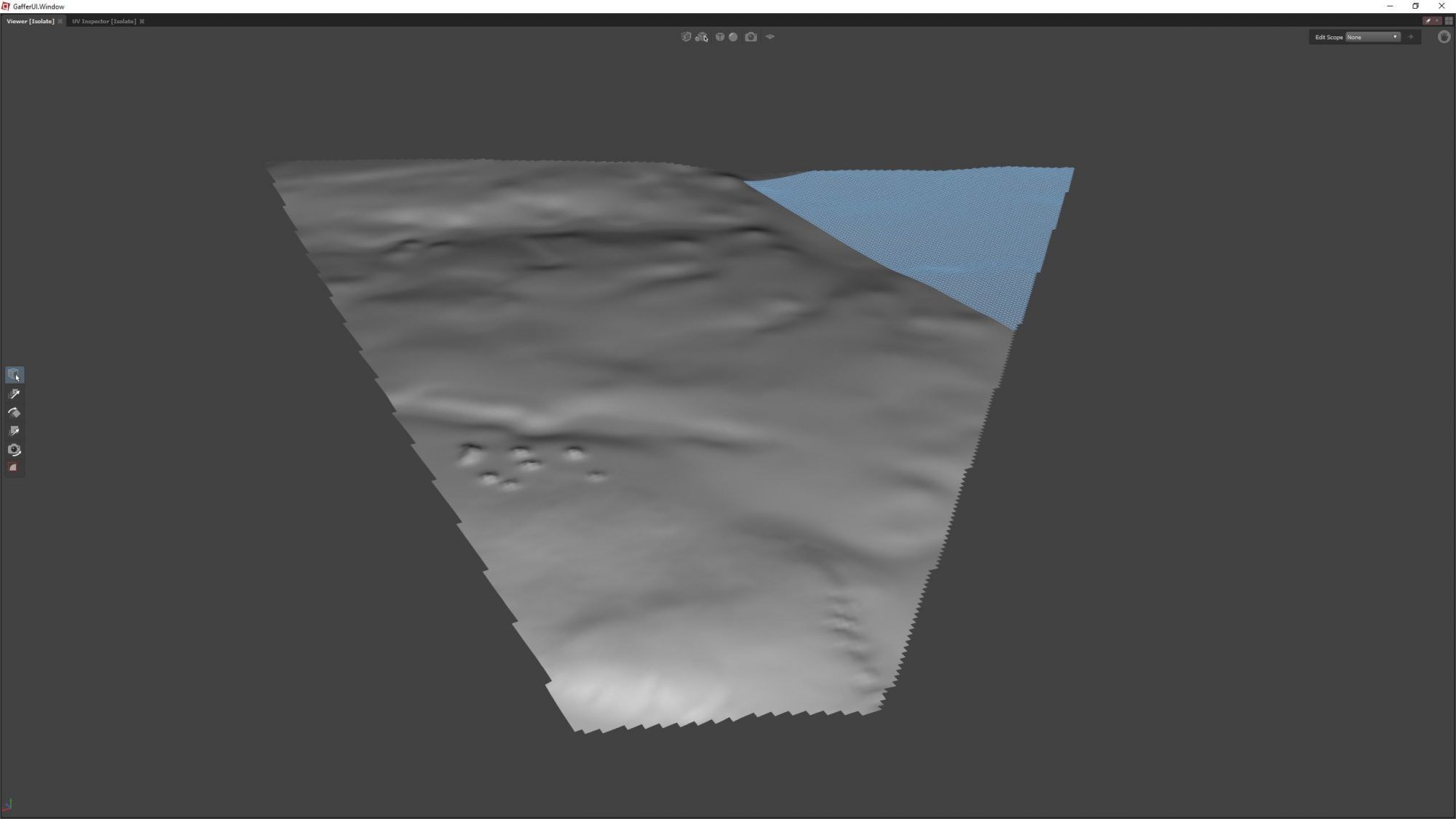
The terrain is then duplicated for the water. The elevation data represents the height of the surface itself, so sampling the water depth and further displacing the terrain by that amount results in the water surface.
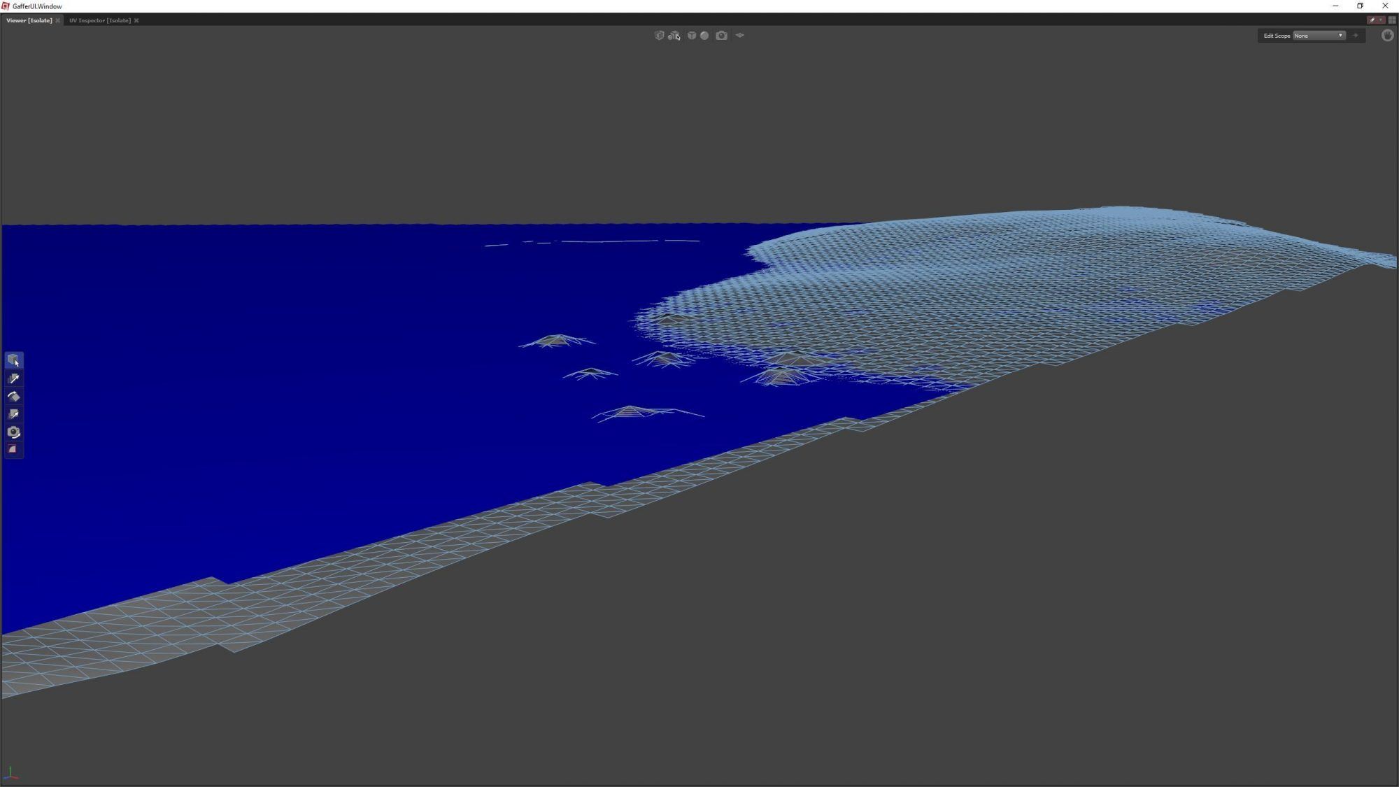
When I started rendering aerial views, a new problem came up. Aerial views can end up including a lot of tiles, often hundreds. For example, a camera 100m above the earth can see about 36km to the horizon. Memory restrictions at that point become a problem.
To solve that, I implemented a simple level of detail system to increase the spacing of grid points of the terrain for tiles farther and farther from the camera. The ImageSampler node works perfectly with this method because it will interpolate image samples for points that don’t lie exactly on a pixel. An expression connected to the plane’s “divisions” setting allows me to tune the detail level based on its distance to the camera and image resolution. Keeping about 2 screen space pixels per division turns out to be a good balance between visual quality and memory usage.
Future development will include a node to implement more sophisticated level of detail techniques to adapt the terrain even better. The water for example can be enormously simplified since it is flat right up until the last couple of triangles that start to overlap the dry land.
Vegetation
With the landscape in place (but not shaded yet, that’s up next) it is time to give attention to the vegetation. There are about 60 different ecosystem types Dr. Sanderson and his team identified. Some are very similar to each other, and some are underwater, but there are still many to populate with plants.
SpeedTree is a great tool for creating vegetation models and it proves to be very useful for creating Welikia plants. They have an extensive library of pre-made models available that serve as a good starting point for further customization. One trait we want to make sure is conveyed is the old-growth nature of the forests. This means not only large trees, but also a wide variation in sizes to represent trees that are relatively younger, having filled in a hole in the forest where a past tree had fallen. I also create variations for the center and edges of the forest. Trees packed in next to each other don’t allow enough light to penetrate lower branches so leaves are concentrated at the top. Trees on the edge of a river bank or other forest edge can get more light down low, so their leaf canopy extends quite low and visually makes for a more impenetrable looking forest.
Although Houdini has good plant scattering capabilities, I ultimately decided to keep the plant distribution within Gaffer. This allows for faster iteration directly in the viewport, easy camera movement to preview different ecosystems, and rendering previews that are critical to getting good results.
Scattering plants in Gaffer is mostly straightforward. Each species is scattered individually using a Seeds node, starting with the dominant species of an ecosystem and working down to smaller scale species. For example, an oak / hickory forest has edge and middle oak tree models, edge and middle hickory models, sapling models for oak and hickory, a scattering of dogwood trees in the understory and a final layer of sparse grass on the ground.
Using a combination of OSLImage nodes, spline widgets, noise maps, blur nodes and image merge nodes, I convert the ecosystem raster data into a probability map for each model ranging from 0-1. The seeds’ elevations are set from an ImageSampler node. A custom node for calculating the gradient of the height map feeds data into Gaffer’s Orientation node for controlling how much the plant will point straight up vs. along the landscape slope.
Each seed also gets a unique ID based on its location so that it will be consistent on each scattering run. Like the terrain tiles, seeds are also culled out of the frustum using a custom node to reduce the data load on the renderer. Without a consistent ID, manual customizations are not possible for moving cameras and would be problematic even for a still camera that may be moved during exploration.
The final step is to cache out the seeds once the plant distributions are looking good. Scattering is fairly quick for a small area, but as with the terrain, aerial views can take prohibitively long to populate, especially for multi-frame animations.
Look Development
Terrain, water and vegetation are all in place now. It’s time to create some shaders! The shaders themselves are pretty straightforward. I chose to use VRay as the render engine. From past experience I know it can handle lots of instancing with low memory consumption. To get it working in Gaffer I needed to code the interface between Gaffer and the VRay AppSDK. I may have more information on that in the future.
A couple parts of the shading configuration are particularly interesting. Using Gaffer’s OSLObject node and a custom node for identifying connected faces, I add data to the tree meshes to vary the leaf colors slightly for each leaf. This adds a subtle but important variation to the trees so they don’t look repetitive.
For the ground, I use the ClosestPoints node again, this time measuring proximity of terrain points to vegetation, to determine what kind of ground texture to apply. Grid points within range of trees get fallen leaf litter textures depending on the species nearest to it. The rest of the points get blended textures based on their dominant ecosystem like mud flats, cliff faces or sandy beaches.
Final Details
Customizing the Scatter
For long aerial views, the procedural scatter does a great job of covering acres of terrain with believable looking vegetation. But when you bring the camera down to ground level, it’s important to be able to add an artistic touch to the layout. You also want to make sure your chosen camera spot isn’t in the middle of a tree.
To allow individual control over trees, a few extra items need to be in place. For one, I need to be able to address a specific tree, regardless of the order in which it was generated. This is because preview renders are often done with a shorter far clipping plane than production renders, and changing using the default Instancer node settings can result in the same tree getting a different name based on it’s placement in the sequence. To sort this, I used the “Id” parameter to add an unique Id, based on an OSLObject hash of the object’s world location, to each instance. Now the instances can be moved, deleted and more based on a constant Id.
Handling High Resolution Trees
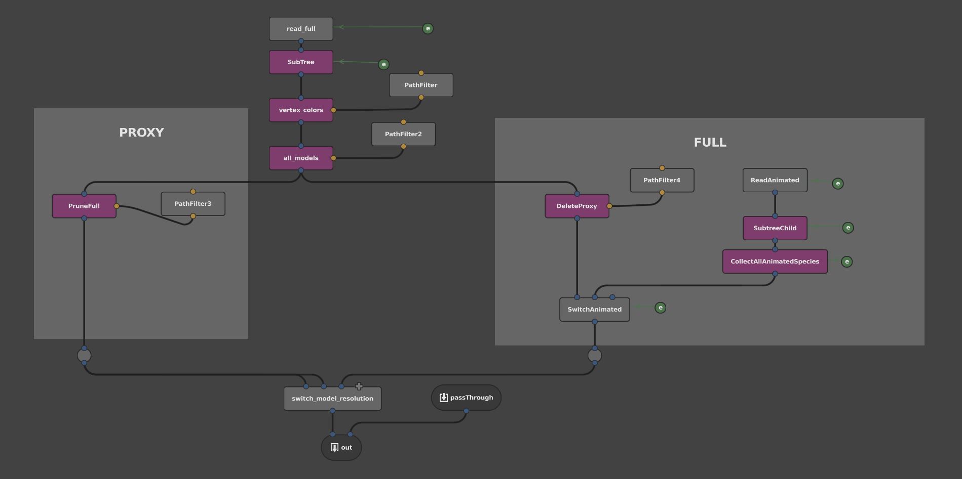
Gaffer’s context variables came to the rescue for simplifying the viewport geometry for trees. With individual trees often having a few million polygons each, it would be a major bottleneck, if it’s possible at all, to load and display the full geometry at all times. But I also needed to make sure that any manual edits to the tree’s location were applied to the proxy and the full resolution tree. Lastly, I wanted to be able to select a tree in the viewport and not risk forgetting to navigate a level up in the hierarchy view before making tweaks.
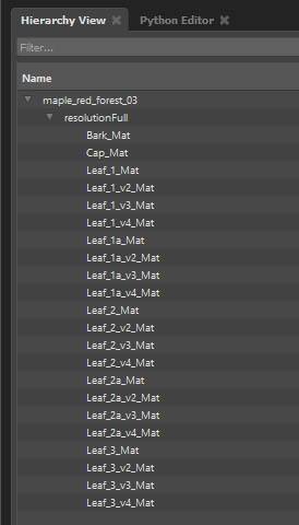
The solution was to create a convex hull for each tree in Houdini, and read that into Gaffer as usual. The full resolution trees were then parented to the proxy. A context variable downstream switches between full resolution and proxy.


Camera Placement
The final piece of the Welikia puzzle is the latitude / longitude based camera locator. For this I use Gaffer’s Expression node to call an external open-source program called proj. Proj handles the intricacies of converting latitude and longitude coordinates to regular cartesian coordinates. It’s a surprisingly difficult problem and one that I’m very happy to delegate to the experts.
I hope you enjoyed that dive into the inner workings of the creation of our Welikia images!